NGS的可视化
我们将用以下的包来说明一下如何对NGS数据进行可视化。
|
|
我们将会采用四种方式来查看NGS的数据,分别是IGV,plot,Gviz和ggbio。
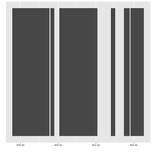
IGV
将这些文献从R library的目录中复制到当前的工作目标。首先将工作目录设置为源文件位置。我们需要使用Rsamtools包来对BAM文件加上索引,然后使用IGV来查看,如下所示:
|
|
IGV可以在这个网站下载: https://www.broadinstitute.org/igv/home
下载的时候需要提供你的电子邮箱,现在我们使用IGV来查看一个基因,例如igs。
如果无法下载IGV,那么可以使用UCSC的 Genome Browser:http://genome.ucsc.edu/cgi-bin/hgTracks
UCSC Genome Browser是一个很好的资源,有许多涉及基因注释,多个物种的保护,以及ENCODE表观遗传信号。但是,UCSC Genome Browser要求你将基因组文件上传到他们的服务器,或将数据放在公共可用服务器上。如果你处理的数据涉及保密,那就另当别论了。
Simple plot
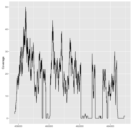
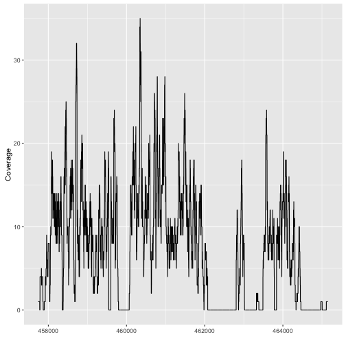
现在我们来看一使用plot()函数来绘制基因。
|
|
注意:如果你使用的是Bioconductor 14,它与R 3.1配合使用,需要加载这个包。如想是Bioconductor 13(它与R 3.0.x配合使用),则不需要加载这个包。
|
|
我们从文件fl1中读取比对结果(alignments)。然后我们使用coverage函数来计算碱基对的覆盖。然后我们提取与我们感兴趣的基因重叠的覆盖区子集,并将此覆盖率从RleList转换为numeric向量。我们前面提到,Rle对象是一种压缩对象,例如重复数字会被压缩为2个数字,其中一个是重复的数字,另外一个是表示这个数字重复的次数。
|
|
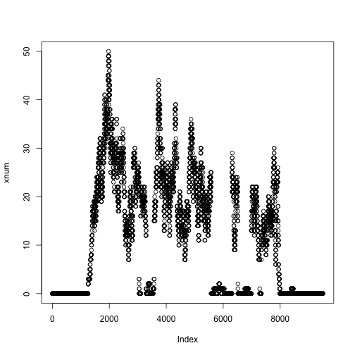
现在我们读取另外一个文件fl2,如下所示:
|
|
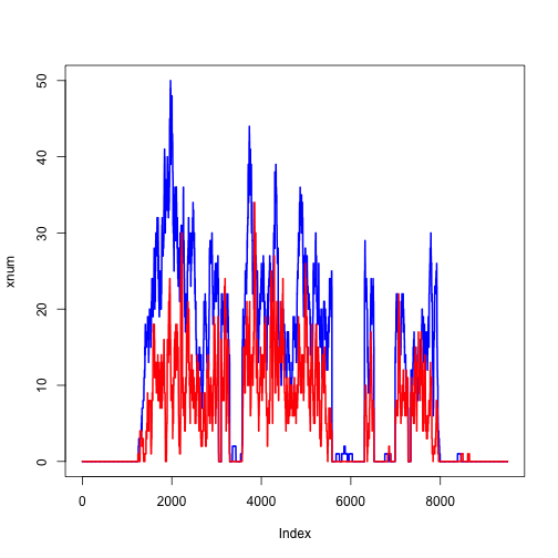
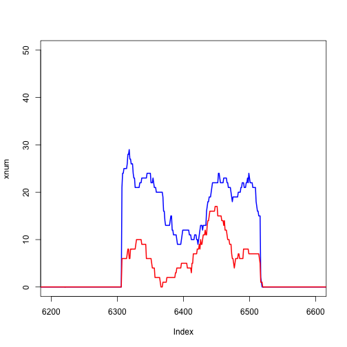
我们可以单独放大一个外显子,如下所示:
|
|
使用转录本数据库提取感兴趣的基因
假设我们想可视化基因igs。我们可以从转录本数据库TxDb.Dmelanogaster.UCSC.dm3.ensGene 中提取它,但我们首先要知道这个基因的Ensembl基因名,现在我们使用前面学到的函数来实现这一功能,如下所示:
|
|
现在我们提取每个基因的外显子,然后提取igs基因的外显子,如下所示:
|
|
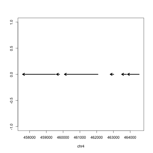
最后,我们绘制出这些外显子的范围,如下所示:
|
|
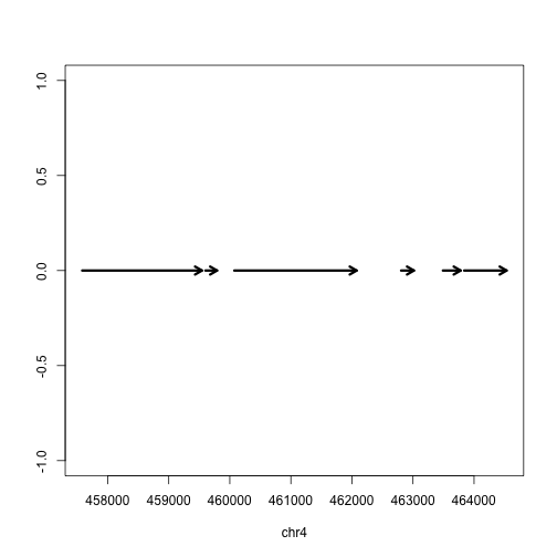
不过实际上这个基因位于负链,因此我们需要改一下箭头的方向,如下所示:
|
|
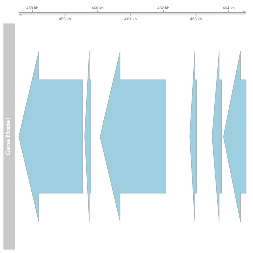
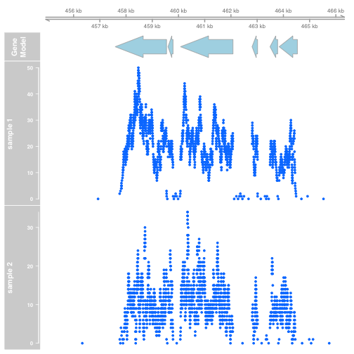
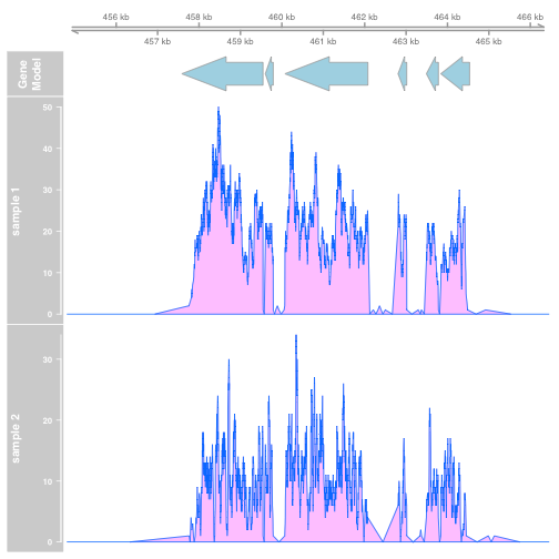
Gviz
我们将简要展示两个在Bioconductor中可视化基因组数据的软件包。请注意,这两个包中的任何一个都可以用于绘制多种数据的图形。我们将在这里展示如何像以前一样制作覆盖图(converage plot):
|
|
提取覆盖。Gviz中的数据最好是是GRanges对象,因此我们需要将RleList转换为GRanges对象,如下所示:
|
|
|
|
ggbio
|
|
|
|
|
|
参考资料
- Visualizing NGS data
- IGV: https://www.broadinstitute.org/igv/home
- Gviz: http://www.bioconductor.org/packages/release/bioc/html/Gviz.html
- ggbio:http://www.bioconductor.org/packages/release/bioc/html/ggbio.html
- UCSC Genome Browser: zooms and scrolls over chromosomes, showing the work of annotators worldwide: http://genome.ucsc.edu/
- Ensembl genome browser: genome databases for vertebrates and other eukaryotic species:http://ensembl.org
- Roadmap Epigenome browser: public resource of human epigenomic data: http://www.epigenomebrowser.org http://genomebrowser.wustl.edu/ http://epigenomegateway.wustl.edu/
- “Sashimi plots” for RNA-Seq: http://genes.mit.edu/burgelab/miso/docs/sashimi.html
- Circos: designed for visualizing genomic data in a cirlce: http://circos.ca/
- SeqMonk: a tool to visualise and analyse high throughput mapped sequence data: http://www.bioinformatics.babraham.ac.uk/projects/seqmonk/